 Colony growth and using ODEs
←Previous tutorial
- Simple colony growth
- Populating the grid with custom, unique individuals
- Displaying a continuous variable on the grid
- Attaching ODEs to grid points
Simple colony growth
For my implementation of colony growth, I used the very simple code shown below:
let randomneigh = this.randomMoore8(this,i,j).alive   // Random neighbour
if(this.grid[i][j].alive == 0)                        // If empty
{
    if(randomneigh == 1 && this.rng.genrand_real1() < 0.5)
        this.grid[i][j].alive = 1                     // 1 ("cell") reproduces
}let config =
{
title: "Colony", // The name of your cacatoo-simulation
description: "", // And a description if you wish
maxtime: 1000000, // How many time steps the model continues to run
ncol: 200, // Number of columns (width of your grid)
nrow: 200, // Number of rows (height of your grid)
seed: 5,
wrap: [false, false], // Wrapped boundary conditions? [COLS, ROWS]
scale: 2, // Scale of the grid (nxn pixels per grid point)
statecolours: {'species': { 1: "#FFFFFF", // Colours for each state. Background (0) defaults to black.
2: "red",
3: "#3030ff"}}
//statecolours: { 'species': 'default' },
}
sim = new Simulation(config) // Initialise the Cacatoo simulation
sim.makeGridmodel("growth") // Build a new Gridmodel within the simulation called "model"
Populating the grid
let species = [{species:1,uptake_rate:0.5,internal_resources:1},
               {species:2,uptake_rate:5.0,internal_resources:1},
               {species:3,uptake_rate:50.0,internal_resources:1}]

sim.populateSpot(sim.growth, species, [0.33,0.33,0.33], 15, config.ncol/2, config.nrow/2)    // Inoculate 1 spot (middle of grid) with species. The third array sets the frequency of each species.
//sim.populateGrid(sim.growth, species, [0.01,0.01,0.01])                                    // Alternatively, inoculate entire grid with species
sim.initialGrid(sim.growth,'external_resources',1000.0,1.0) // Add 1000.0 external resources to 100% (1.0) of grid points
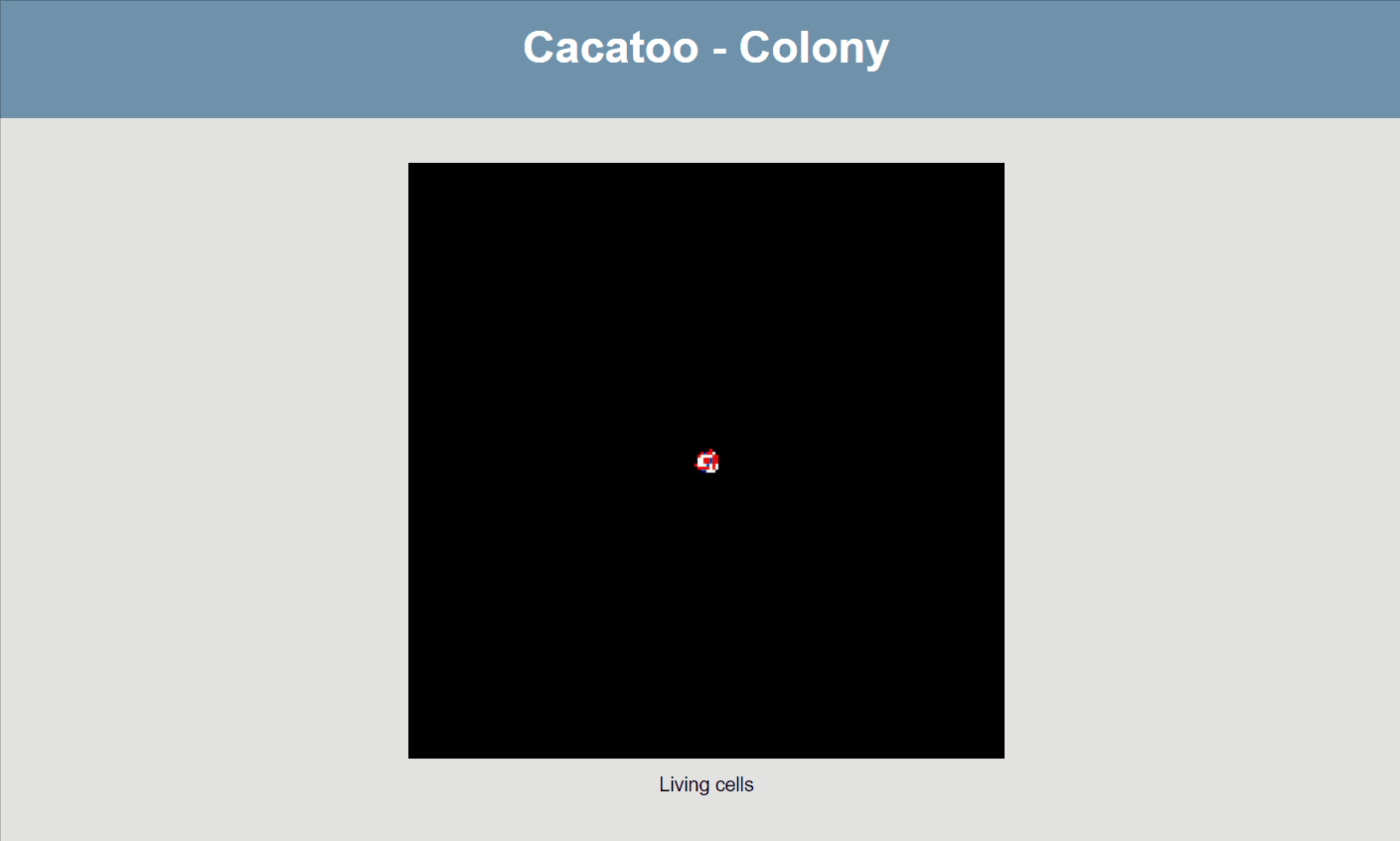
sim.createDisplay("growth", "species", "Living cells") // Create a display in the same way we did in Tutorial 1 (display a discrete variable)
sim.growth.nextState = function (i, j) {
let randomneigh = this.randomMoore8(this, i, j)   // Random neighbour
let this_gp = this.grid[i][j]                     // This cell

if (this_gp.species == 0)                        // If empty spot
{
    if (randomneigh.species > 1 && randomneigh.internal_resources > 50) {   // Random neighbour is alive and it has enough resources
        this_gp.species = randomneigh.species                               // Empty spot becomes the parent type (reproduction)
        this_gp.uptake_rate = randomneigh.uptake_rate                       // Empty spot inherits uptake rate from the parent
        randomneigh.internal_resources = this_gp.internal_resources = randomneigh.internal_resources / 2    // Resources are divided between parent and offpsring
    }
}
else {
    if (this.rng.genrand_real1() < 0.01) {                                      // Random death
        this_gp.species = 0
        this_gp.uptake_rate=0.0
        this_gp.internal_resources = 0
    }
    else{
        let uptake = this_gp.external_resources * (this_gp.uptake_rate/100)     // Living cells can take up a fraction of available resources
        this_gp.internal_resources += uptake
        this_gp.external_resources -= uptake
    }
}
}
If all goes well, your simulation should now look like this:
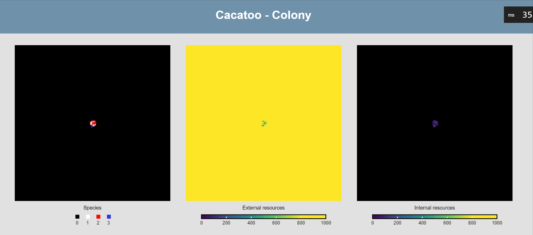
The simulation shows that the blue species (high uptake rate) is growing much faster than the red one, and that the white species isn't able to really grow at all! However, it would be better if we could actually see the resource concentrations, both inside and outside of cells.
Displaying a continuous variable
sim.createDisplay_continuous({model:"growth", property:"external_resources", label:"External resources", // Createa a display for a continuous variable (ODE state for external resources)
                minval:0, maxval:1000, fill:"viridis"})
sim.createDisplay_continuous({model:"growth", property:"internal_resources", label:"Internal resources", // Createa a display for a continuous variable (ODE state for external resources)
minval:0, maxval:1000, fill:"viridis"})If all goes well, you should now see this:
Attach ODEs to grid points
// Define ODEs with basic resource dynamics
let resource_dynamics = function (u, k) {
    return function (x, y) {
        let external = y[0] // The first variable (y[0]) is the external resource concentration, which is taken up with rate u
        let internal = y[1] // The second variable (y[1]) is the internal resource concentration, which is used by the cells to divide
        return [   -u * external,
                    u * external - k * internal ]
    }
}
// Configuration object with initial states, parameters, and diffusion rates
let ode_config = {
    ode_name: "resources",
    init_states: [1, 0],              // Initial values of external and internal resources
    parameters: [0.0, 0.0],           // u and k are set to 0.0 by default, as we will make it dependent on cell presence!
    diffusion_rates: [0.2, 0.0]       // resources diffuse through exteral environment, but internal resources stay inside cells
}

// Attaches an ODE to all gridpoints with the given configuration object
sim.model.attachODE(resource_dynamics, ode_config);sim.model.nextState = function (i, j)
{
let randomneigh = this.randomMoore8(this, i, j) // Random neighbour
let this_gp = this.grid[i][j] // This cell
if (this_gp.species == 0) // If empty
{
if (randomneigh.species > 1 && randomneigh.resources.state[1] > 0.5) {
this_gp.species = randomneigh.species
this_gp.uptake_rate = randomneigh.uptake_rate
randomneigh.resources.state[1] = this.grid[i][j].resources.state[1] = randomneigh.resources.state[1] / 2
}
}
else {
this.grid[i][j].resources.pars = [this_gp.uptake_rate, 0.5] // Living cells take up and have upkeep
if (this.rng.genrand_real1() < 0.01) {
this_gp.species = 0
this_gp.uptake_rate=0.0
this_gp.resources.state[1] = 0
this_gp.resources.pars = [0.0, 0.0]
}
}
this_gp.resources.solveTimestep(0.1) // Solve a single time step with delta_t=0.1
this_gp.external_resources = this_gp.resources.state[0]
if(this_gp.species > 0) this_gp.internal_resources = this.grid[i][j].resources.state[1]
else this.grid[i][j].rersources = 0.0
}
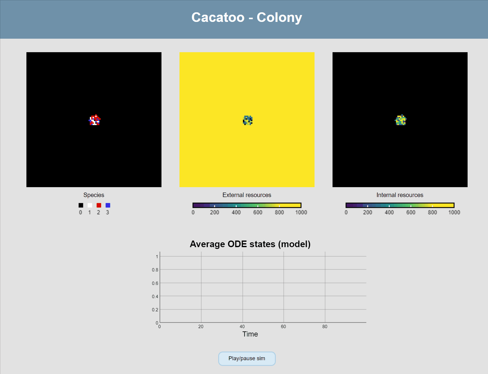
And one final thing we want to do is modify the main update-loop to add diffusion of the ODE states between grid points (i.e. the external resources), and add a plot so we can see the concentrations changing:
    sim.model.update = function () {
        this.asynchronous()         // Applied as many times as it can in 1/60th of a second
        this.diffuseODEstates()       // Diffusion of external metabolites
        this.plotODEstates("resources", [0, 1], [[0, 0, 0], [255, 0, 0]])
} 
And that wraps up this series of tutorials. The end-result of the tutorials can be found on the Github repository. If you want to learn more, start exploring the many examples available there.